: No 7. PIME Analysis

Setup

First, we grab the whole community, fish only, phyloseq object.

ps.whole <- readRDS("rdata/p3/ps_16S_bocas_fish_final.rds")

ps.whole <- phyloseq(otu_table(ps.whole), sample_data(ps.whole), tax_table(ps.whole))
ps.whole@phy_tree <- NULL

phyloseq-class experiment-level object
otu_table()   OTU Table:         [ 3113 taxa and 89 samples ]
sample_data() Sample Data:       [ 89 samples by 11 sample variables ]
tax_table()   Taxonomy Table:    [ 3113 taxa by 11 taxonomic ranks ]

Next, we calculate the baseline noise detection

pime.oob.error(ps.whole, "Zone")

And then split by Zone (i.e., Inner bay disturbed, Inner bay, & Outer bay).

data.frame(sample_data(ps.whole))
per_variable_obj <- pime.split.by.variable(ps.whole, "Zone")
per_variable_obj

$`Inner bay`
phyloseq-class experiment-level object
otu_table()   OTU Table:         [ 1590 taxa and 35 samples ]
sample_data() Sample Data:       [ 35 samples by 11 sample variables ]
tax_table()   Taxonomy Table:    [ 1590 taxa by 11 taxonomic ranks ]

$`Inner bay disturbed`
phyloseq-class experiment-level object
otu_table()   OTU Table:         [ 909 taxa and 19 samples ]
sample_data() Sample Data:       [ 19 samples by 11 sample variables ]
tax_table()   Taxonomy Table:    [ 909 taxa by 11 taxonomic ranks ]

$`Outer bay`
phyloseq-class experiment-level object
otu_table()   OTU Table:         [ 1271 taxa and 35 samples ]
sample_data() Sample Data:       [ 35 samples by 11 sample variables ]
tax_table()   Taxonomy Table:    [ 1271 taxa by 11 taxonomic ranks ]

Calculate the Prevalence Intervals

Using the output of pime.split.by.variable, we calculate the prevalence intervals with the function pime.prevalence. This function estimates the highest prevalence possible (no empty ASV table), calculates prevalence for taxa, starting at 5 maximum prevalence possible (no empty ASV table or dropping samples). After prevalence calculation, each prevalence interval are merged.

prevalences <- pime.prevalence(per_variable_obj)
head(prevalences)

$`5`
phyloseq-class experiment-level object
otu_table()   OTU Table:         [ 1143 taxa and 89 samples ]
sample_data() Sample Data:       [ 89 samples by 11 sample variables ]
tax_table()   Taxonomy Table:    [ 1143 taxa by 11 taxonomic ranks ]

$`10`
phyloseq-class experiment-level object
otu_table()   OTU Table:         [ 266 taxa and 89 samples ]
sample_data() Sample Data:       [ 89 samples by 11 sample variables ]
tax_table()   Taxonomy Table:    [ 266 taxa by 11 taxonomic ranks ]

$`15`
phyloseq-class experiment-level object
otu_table()   OTU Table:         [ 118 taxa and 89 samples ]
sample_data() Sample Data:       [ 89 samples by 11 sample variables ]
tax_table()   Taxonomy Table:    [ 118 taxa by 11 taxonomic ranks ]

$`20`
phyloseq-class experiment-level object
otu_table()   OTU Table:         [ 76 taxa and 89 samples ]
sample_data() Sample Data:       [ 89 samples by 11 sample variables ]
tax_table()   Taxonomy Table:    [ 76 taxa by 11 taxonomic ranks ]

$`25`
phyloseq-class experiment-level object
otu_table()   OTU Table:         [ 57 taxa and 89 samples ]
sample_data() Sample Data:       [ 89 samples by 11 sample variables ]
tax_table()   Taxonomy Table:    [ 57 taxa by 11 taxonomic ranks ]

$`30`
phyloseq-class experiment-level object
otu_table()   OTU Table:         [ 42 taxa and 89 samples ]
sample_data() Sample Data:       [ 89 samples by 11 sample variables ]
tax_table()   Taxonomy Table:    [ 42 taxa by 11 taxonomic ranks ]

Calculate the Best Prevalence

Finally, we use the function pime.best.prevalence to calculate the best prevalence. The function uses randomForest to build random forests trees for samples classification and variable importance computation. It performs classifications for each prevalence interval returned by pime.prevalence. Variable importance is calculated, returning the Mean Decrease Accuracy (MDA), Mean Decrease Impurity (MDI), overall and by sample group, and taxonomy for each ASV. PIME keeps the top 30 variables with highest MDA each prevalence level.

set.seed(1911)
best.prev <- pime.best.prevalence(prevalences, "Zone")

Looks like the lowest OOB error rate (%) is 2.25% from Prevalence 65%. We will use this interval.

imp65 <- best.prev$`Importance`$`Prevalence 65`
write.csv(imp65, file = "tables/p7/output_PIME_Zone65.csv")

Best Prevalence Summary

Now we need to create a phyloseq object of ASVs at this cutoff (Prevalence 65%).

prevalence.65 <- prevalences$`65`
summarize_phyloseq(prevalence.65)
saveRDS(prevalence.65, "rdata/p7/Pime_Prevalence_65.rds")

And look at a summary of the data.

phyloseq-class experiment-level object
otu_table()   OTU Table:         [ 17 taxa and 89 samples ]
sample_data() Sample Data:       [ 89 samples by 11 sample variables ]
tax_table()   Taxonomy Table:    [ 17 taxa by 11 taxonomic ranks ]

Metric	Results
Min. number of reads	288
Max. number of reads	10277
Total number of reads	561593
Average number of reads	6310
Median number of reads	6703
Median number of reads	6703
Sparsity	0.577
Total ASVS	17

Estimate Error in Prediction

Using the function pime.error.prediction we can estimate the error in prediction. For each prevalence interval, this function randomizes the samples labels into arbitrary groupings using n random permutations, defined by the user. For each, randomized and prevalence filtered, data set the OOB error rate is calculated to estimate whether the original differences in groups of samples occur by chance. Results are in a list containing a table and a box plot summarizing the results.

randomized <- pime.error.prediction(ps.whole, "Zone", bootstrap = 100,
                                    parallel = TRUE, max.prev = 95)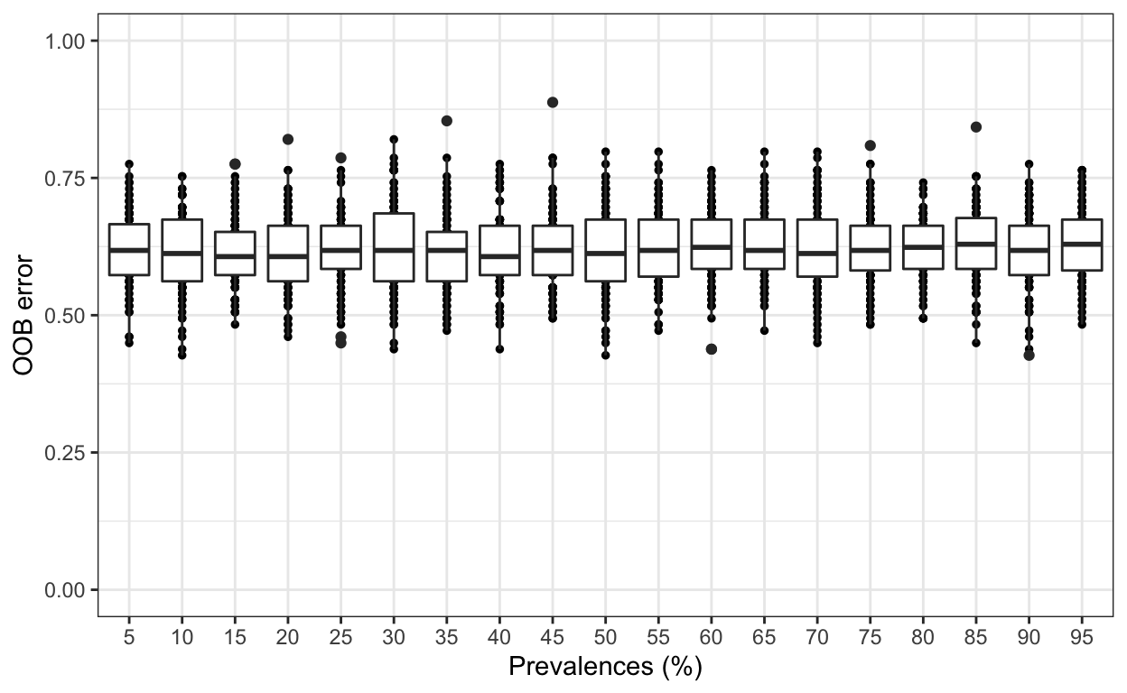

It is also possible to estimate the variation of OOB error for each prevalence interval filtering. This is done by running the random forests classification for n times, determined by the user. The function will return a box plot figure and a table for each classification error.

replicated.oob.error <- pime.oob.replicate(prevalences, "Zone",
                                         bootstrap = 100, parallel = TRUE)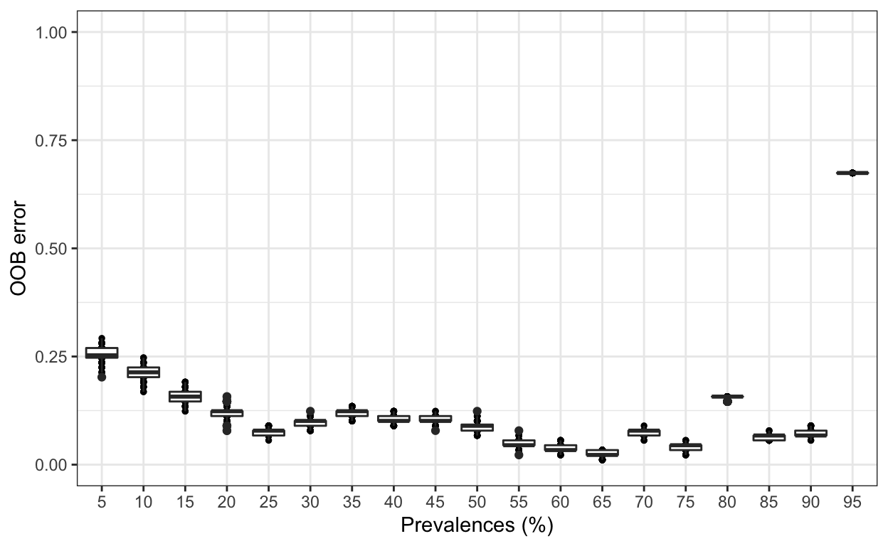

To obtain the confusion matrix from random forests classification use the following:

best.prev$Confusion$`Prevalence 65`

                    Inner bay Inner bay disturbed Outer bay
Inner bay                  34                   0         1
Inner bay disturbed         0                  18         1
Outer bay                   0                   0        35
                    class.error
Inner bay            0.02857143
Inner bay disturbed  0.05263158
Outer bay            0.00000000

Distribution of PIME ASVs across Samples

per_zone = pime.split.by.variable(prevalence.65, "Zone")
per_zone

$`Inner bay`
phyloseq-class experiment-level object
otu_table()   OTU Table:         [ 12 taxa and 35 samples ]
sample_data() Sample Data:       [ 35 samples by 11 sample variables ]
tax_table()   Taxonomy Table:    [ 12 taxa by 11 taxonomic ranks ]

$`Inner bay disturbed`
phyloseq-class experiment-level object
otu_table()   OTU Table:         [ 9 taxa and 19 samples ]
sample_data() Sample Data:       [ 19 samples by 11 sample variables ]
tax_table()   Taxonomy Table:    [ 9 taxa by 11 taxonomic ranks ]

$`Outer bay`
phyloseq-class experiment-level object
otu_table()   OTU Table:         [ 7 taxa and 35 samples ]
sample_data() Sample Data:       [ 35 samples by 11 sample variables ]
tax_table()   Taxonomy Table:    [ 7 taxa by 11 taxonomic ranks ]

Finally, we can create a stacked bar chart for the PIME obtained.

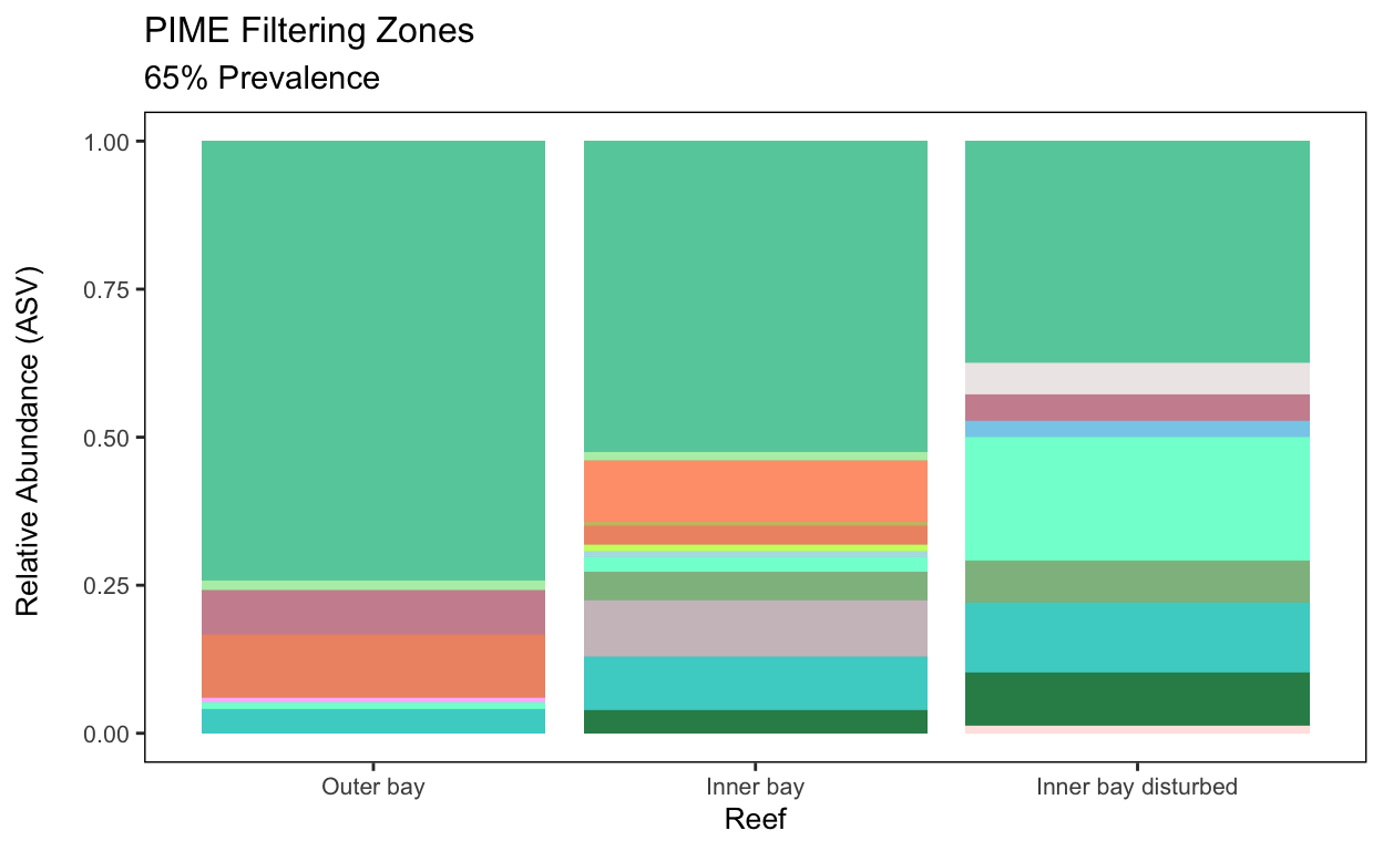
That’s the end of Script 7 and the entire workflow. Thanks for stopping by!

Source Code

The source code for this page can be accessed on GitHub by clicking this link.

No 7. PIME Analysis